ORCA Science Special #4: machine learning

It’s time for more data exploration, so for today’s blog ORCA Data Analyst Ellie K investigates how we might go about identifying fin whale habitat along the Bay of Biscay ferry routes using machine learning methods.

If you’ve opened a news website since the advent of ChatGPT towards the end of 2022, you will doubtless have seen many an alarmist opinion piece on how AI is bad news for you, your job, your children, democracy and humanity in general. While the possible nefarious uses are many, did you know that machine learning models (of which AI is a subset) can help us get a bit of an insight into cetacean ecology and contribute to conservation? What a time to be alive!

Those of you who keep up with ORCA’s work may be aware that one of our big projects is understanding fin whale behaviour in close proximity to large vessels in the Bay of Biscay. As well as this cutting-edge field research, it’s also important to understand where whales are likely to reside so ships can take action before they get close enough that the whales need to get out of the way (if they can) (1).

One way to try and work this out is to quantify the relationship between whale occurrence and habitat features and then extrapolate this relationship to predict where else whales might be. This is a field of ecology known as species distribution modelling (see 10 for a nice introduction to the topic) and is a favourite topic of mine. Machine learning methods are often used to carry it out, so for today’s science blog, we are going full nerd to see how these techniques might be applied to predicting fin whale habitat along the ferry routes we survey in the Bay of Biscay.

To start with, it helps to have a bit of an idea about what kind of things you might expect to affect fin whale distribution as well as large whale distribution more generally and for that, the scientific literature is a good place to start. What you don’t want to do is use as many variables as you can get your hands on as you risk finding spurious relationships and ending up with a bulky and cumbersome model that is difficult to actually interpret and probably won’t generalise to new data very well. An important principle therefore is parsimony, i.e. the simpler the analysis, the better so we want to make sure we are only using variables that are likely to be relevant. Sometimes it helps to summarise what you find in the literature in a little table to help you organise your thoughts. Here’s one I made earlier:

A non-exhaustive summary of some of the things that have been related to baleen whale occurrence in a handful of previous studies

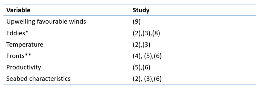
* An eddy is a rotating area of water. A brief introduction to these can be read here. Eddies can aggregate weakly swimming organisms and attract their predators.

**A front is an interface between contrasting water masses, e.g. between warm and cool water or between fast flowing and slow flowing water to name just two examples.

Fin whales in the northeast Atlantic are known to eat krill (11) and canyons can support high densities of krill (12) so let’s also include a variable describing the distance of a data point from the nearest canyon. Fortunately, this kind of information is publicly available and the data can be found here: (13,14,15). I got the oceanographic data at the monthly scale to start with to speed up the processing time. The ocean is always on the move, however, and consequently, some of these variables differ substantially over time. To keep it simple for now, let’s just consider the average of the oceanographic variables during the survey season over time. I also obtained the average gradient in sea surface temperature (SST) using this R package (16) to include the effects of thermal fronts and calculated the eddy kinetic energy from the northward and eastward current velocity as described in this paper (17). There can also be time lags between environmental conditions and an effect on whales since these changes have to propagate through a few trophic levels first (9), so I have included the average chlorophyll during the spring months to try and account for lags between increased productivity in the spring and whale distribution.

Another important consideration in any species distribution model is the scale or alternatively grain size of the analysis. This is a whole blog topic of its own so I will point those readers interested to (7) for now and for simplicity I will resample all of my environmental layers to the same resolution as the coarsest environmental variable, in this case about 7.5 kilometres squared. This means we will be predicting the presence of whales in each 7.5 kilometre grid cell of our study area.

Let’s do a little bit of cleaning up first too. Those of you who have done your Marine Mammal Surveyor course will know the importance of recording sea state and other environmental conditions because of their impact on our ability to detect animals if present, so we will only keep effort and sightings data in sea state 5 or less and in visibility of more than 500 metres. This should prevent data collected in conditions that would make it difficult to spot a whale if it were really there from affecting our conclusions. We will also only keep definite fin whales and sightings made within a sensible distance of the ship so we can be extra confident about species ID. This leaves us with 525 sightings. I have checked beforehand how representative the habitat on the ferry routes is of the environmental conditions in the Bay of Biscay as a whole using the method described in (18) and it looks pretty representative so hopefully we can ignore any potential bias caused by surveying from platforms of opportunity. Since data collection protocols have been consistent since 2014, I will only use data since then and until 2022 for reasons that will shortly become clear.

Now that we have worked out which variables might be good predictors of whale occurrence, tracked down the data for them and cleaned up our sightings and effort data, we now need to decide: which model should we use?

We are spoilt for choice here and there are as many ways to try and predict fin whale occurrence as there are to cuddle a cat. This blog is about machine learning though, so that rules out traditional regression-based techniques like GLM and GAM. One of the great advantages of machine learning techniques over these statistical models is that they don’t make any assumptions about the data to begin with and learn from the data as it is, which is a big plus for data on species distributions which often do not conform to the very prescriptive assumptions of statistical models (20).

As well as sightings, we also have that all important effort data which can give us an idea of where whales are not seen, so models that only use presences are also out at this stage. This still leaves us with an overwhelming choice of models (check out 19 for an overview of applications of machine learning in marine ecology if that kind of thing tickles your fancy) so I will cut to the chase and suggest the boosted regression tree. In short, the idea here is to keep building small models that each have a little bit of explanatory power on top of each other to get one big model that explains as much variation in the data as possible while also paying special attention to observations that prove difficult to classify correctly. The interested reader may refer to these references for the nitty gritty (20,21). These models are a popular choice as they tend to do a good job at predicting things (21), although unless we’re careful about how we run them they are prone to overfitting (22).

Overfitting means that the model hugs to the data points too closely and although a model that has been overfitted does an excellent job of describing the data we used to build it, it is too specific to be any good at predicting to new data, so we will need to beware of overfitting as our goal is to predict after all.

Even though we have settled on our model, we still have a few more choices to make regarding settings. The key ones for a boosted regression tree are the learning rate and the tree complexity. These govern how much each of the individual little models contributes to the final model and how complex we want the interactions between explanatory variables to be respectively. I like things simple, so I will limit the tree complexity to two so we will only get two way interactions and I will have a better chance of interpreting what they mean. For the uninitiated, interactions tell you whether the effect of one variable depends on another and if so, how. I played around with the learning rate and arrived at 0.005 as a reasonable value for this exploratory analysis. I used the dismo package in the statistical programming environment R to do the actual modelling (23).

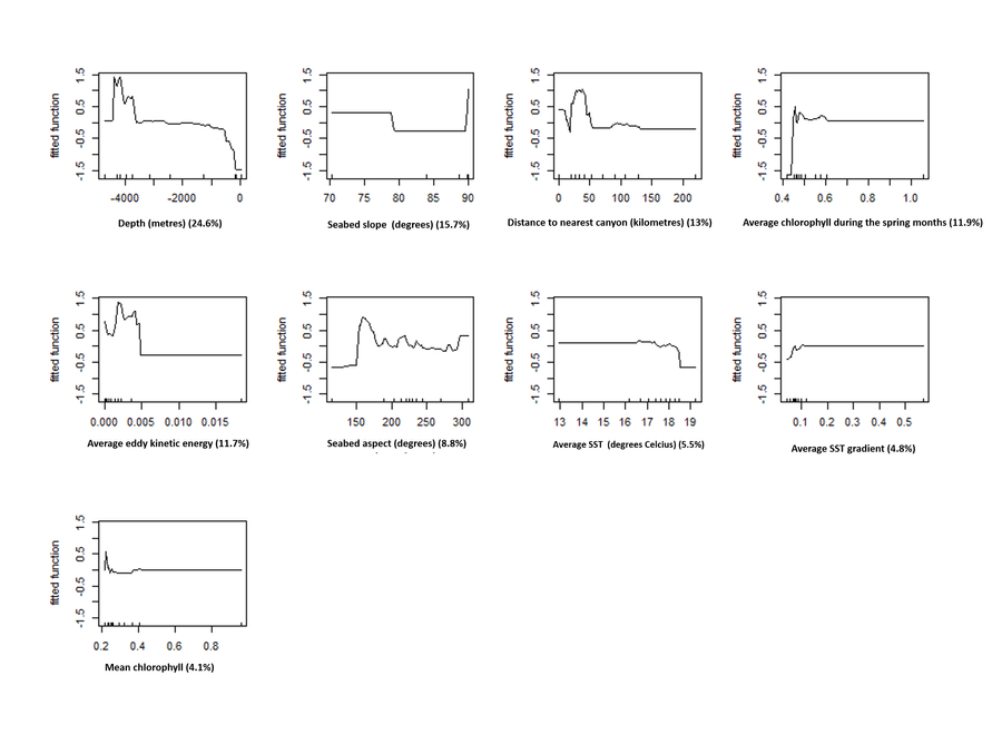
Ok, so what does this model show? For starters, here is the order of the variables we used from most to least important: depth, slope, distance from the nearest canyon, mean chlorophyll during the spring months, eddy kinetic energy, aspect, mean SST, mean SST gradient and mean chlorophyll overall. This model has an AUC statistic (a measure of predictive accuracy, specifically the ability to correctly distinguish presences from absences and vice versa) of 0.9 which is pretty good (24)!

We can see what kind of relationship fin whale presence has with each variable by looking at the partial dependence plot shown below. These just show you how the presence of whales on the y axis responds to values of the variable on the x axis when the values of all the other variables in the model are held at their average value. It would seem that fin whale presence is highest at depths >3000 metres, at both low slope values and very high slope values, close to canyons and in areas where spring chlorophyll was pretty low. You may notice that the least informative variables, mean chlorophyll and average SST gradient are more or less flat.

That’s all well and good and definitely very interesting, but how do we know that this model is actually any good at identifying areas with whales?

Well, we can test it with some data it hasn’t seen before and see how accurate it is. Before I did the above, I kept 25% of the dataset behind and it is this data that we can use to evaluate the model we just built. In an ideal world, we would have a completely independent dataset to use for this (25). Given this withheld data, the AUC went down to 0.84, which, although a drop from the score for the initial model, is still pretty accurate. For reference, an AUC score of 0.8 or more is considered excellent (24) so our model is good according to this measure.

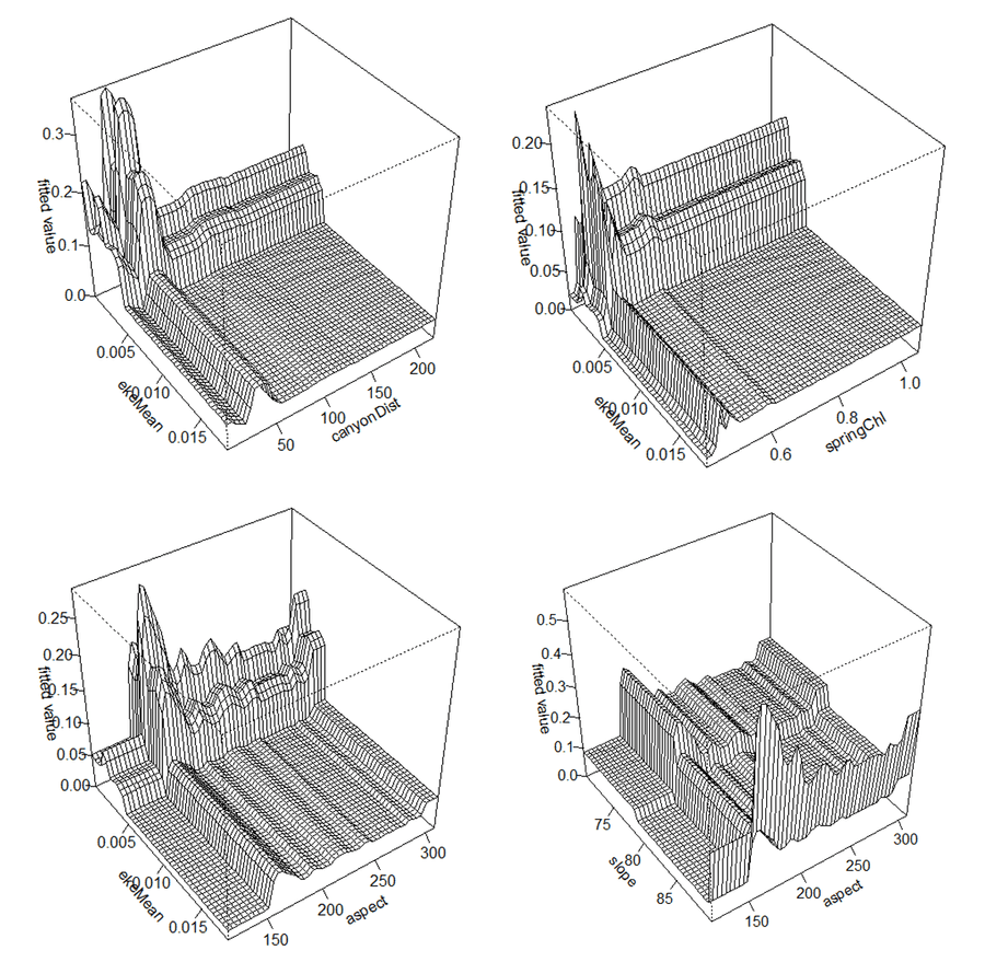
What about interactions? The important ones are shown below. The majority of these involve eddy kinetic energy and low values of it, with higher presence predicted in less energetic areas close to canyons, in areas with low energy and low chlorophyll during the spring and in areas with low energy and a south facing seabed. There is also an interaction between slope and aspect with higher presence on steep, south facing areas of seabed.

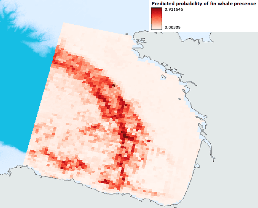
So now we have an idea of which of our variables are most strongly related to fin whale occurrence on average. Next, we need to use the results of this model to predict in space if our goal is to find out where we might find a whale based on these modelled relationships. This is easily done in R and our prediction is shown below. It looks like this model predicts the highest presence of fin whales in the canyons and along the seaward edge of the continental slope and minimal presence over the shallow continental shelf and the very deepest, flattest abyssal plain.

At this point, we have another opportunity to test our model’s predictive capacity by giving it the environmental data for a year not included in the model - 2023 - and asking it to predict where the best whale habitat would have been last year based on the model built with 2014-2022’s data. We can then use the actual 2023 sightings to eyeball how well it did. So?

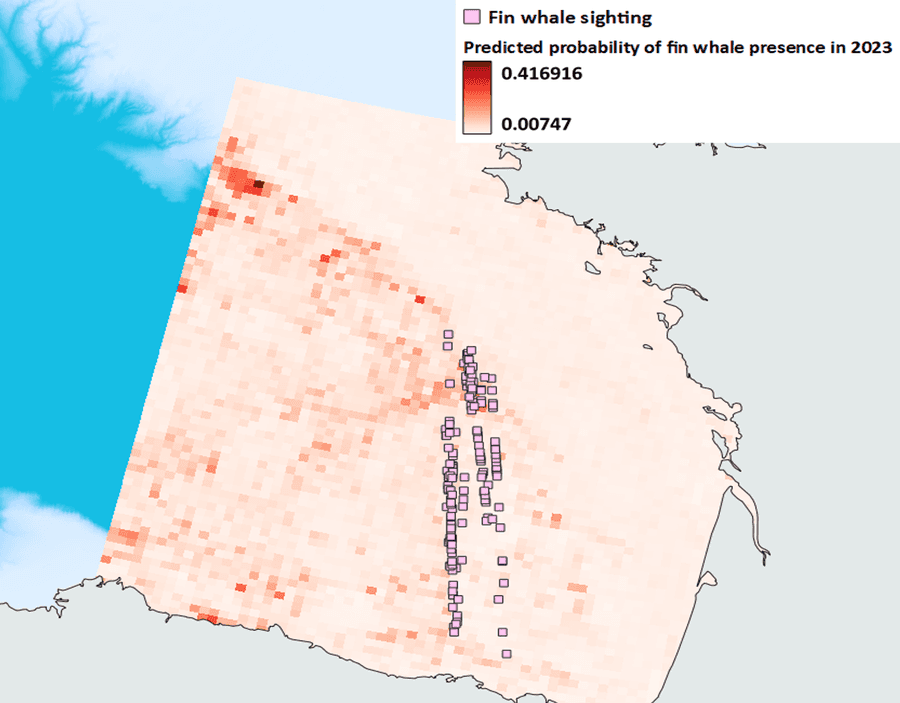
Uh oh, that doesn’t look quite right. 2023 was a pretty warm year in the Bay of Biscay and consequently, the temperature is slightly higher than the average temperature data we used to build the model so it predicts more whale habitat far to the northwest where it was cooler, despite the fact there were still plenty of whales to be seen in the usual places. Notice also how the absolute values of presence are pretty low in the top left corner when in fact 2023 was a good year for sightings. Back to the drawing board?

What does this all mean?

Overall, the static variables like depth and slope were the most important and the more variable variables (try saying that five times fast) like temperature were less important. This makes sense, since as the name implies, these static features stay the same over time so they could be predictable foraging habitats. Returning to these features time and again could save a hungry whale a lot of time and energy. Remember though that we have taken an average of the oceanographic variables over the entire study period and if we examined the importance of these variables closer to the time of unique sightings, we might get a very different picture (26). Hold that thought for later. Indeed, our experiment with 2023’s environmental data has shown that the long-term average of these variables might not give us a good prediction for future years and as things are set to warm up with, we need our predictions to be robust to future changes in environmental conditions (27).

And finally, where do we go from here?

A really useful tool in vessel strike mitigation and the management of other threats is modelling to predict where high densities of whales are likely to be found RIGHT NOW - a concept known as dynamic ocean management (28). This has already been developed in other areas including California and New Zealand (29,30). A possible next step from here would be to revamp this model to predict fin whale occurrence at finer scales to forecast fin whale distribution in the Bay of Biscay in a similar way. A tantalising prospect! But I might need a bit more computing power.

That's all from me! Ellie K, ORCA Data Analyst

References:

(1) Redfern, J.V., McKenna, M.F, Moore, T.J., Calambokidis, J., Deangelis, M.L., Becker, E.A., Barlow, J., Forney, K.A., Fielder, P.C. and Chivers, S.J. (2013). Assessing the risk of ships striking large whales in marine spatial planning. Conservation Biology 27:292-302

(2) Garcia-Baron, I., Authier, M., Caballero, A., Vazquez, J.A., Santos, M.B., Murcia, J.L., Louzao, M. (2019). Modelling the spatial abundance of a highly migratory predator: a call for transboundary marine protected areas. Diversity and Distributions 25(3): 346-360

(3) Perez-Jorge, S., Tobena, M., Prieto, R., Vandeperre, F., Calmettes, B., Lehodey, P., and Silva, M.A. (2019). Environmental drivers of large-scale movements of baleen whales in the mid-North Atlantic Ocean. Diversity and Distributions 26(6): 683-698

(4) Abrahms, B., Welch, H., Brodie, S., Jacox, M.G., Becker, E.A., Bograd, S.J., Irvine, L.M., Palacios, D.M., Mate, B.R. and Hazen, E.L. (2019). Dynamic ensemble models to predict distributions and anthropogenic risk exposure for highly mobile species. Diversity and Distributions 25(8): 1182-1193

(5) Druon, J., Panigada, S., David, L., Gannier, A., Mayol, P., Arcangeli, A., Canadas, A., Laran, S., Di Meglio, N. and Gauffier, P. (2012). Potential feeding habitat of fin whales in the western Mediterranean Sea: an environmental niche model. Marine Ecology Progress Series 464: 289-306

(6) Scales, K.L., Schorr, G.S., Hazen, E.L., Bograd, S.J., Miller, P.I., Andrews, R.D., Zerbini, A.N. and Falcone, E.A. (2017). Should I stay or should I go? Modelling year-round habitat suitability and drivers of residency for fin whales in the California Current. Diversity and Distributions 23: 1204-1215

(7) Guisan, A., Graham, C.H., Elith, J. and Huettmann, F. (2007). Sensitivity of predictive species distribution models to changes in grain size. Diversity and Distributions 13: 332-340

(8) Cotte, C., d’Ovidio, F., Chaigneau, A., Levy, M., Taupier-Letage, Mate, B., and Guinet, C. (2011). Scale-dependent interactions of Mediterranean whales with marine dynamics. Limonology and Oceanography 56(1): 219-232

(9) Barlow, D.R., Klinck, H., Ponirakis, D., Garvey, C. and Torres, L.G. (2021). Temporal and spatial lags between wind, coastal upwelling and blue whale occurrence. Scientific Reports 11:6915

(10) Elith, J. and Leathwick, J.R. (2009). Species distribution models: ecological explanation and prediction across space and time. Annual Review of Ecology, Evolution and Systematics 40: 677-697

(11) Ryan, C., Berrow, S.D., McHugh, B., O’Donnell, C., Trueman, C.N. and O’Connor, I. (2014). Prey preferences of sympatric fin (Balaenoptera physalus) and humpback (Megaptera novaeangliae) whales revealed by stable isotope mixing models. Marine Mammal Science 30(1): 242-258

(12) Santora, J.A., Zeno, R., Dorman, J.G. and Sydeman, W.J. (2018). Submarine canyons represent an essential habitat network for krill hotspots in a Large Marine Ecosystem. Scientific Reports 8:7579

(13) Harris, P.T., Macmillan-Lawler, M., Rupp, J. and Baker, E.K. (2014). Geomorphology of the oceans. Marine Geology 352: 4-24

(14) Atlantic-Iberian Biscay Irish- Ocean Physics Reanalysis. E.U. Copernicus Marine Service Information (CMEMS). Marine Data Store (MDS). DOI: https://doi.org/10.48670/moi-0... . (Accessed on 09/05/2024)

(15) Atlantic-Iberian Biscay Irish- Ocean Biogeochemical Analysis and Forecast. E.U. Copernicus Marine Service Information (CMEMS). Marine Data Store (MDS). DOI: https://doi.org/10.5194/os-15-.... (Accessed on 09/05/2024)

(16) Lau-Medrano, W. (2020). grec: Gradient-based recognition of spatial patterns in environmental data. R package version 1.4.1.

(17) Hobday, A.J. and Hartog, J.R. (2014). Derived ocean features for dynamic ocean management. Oceanography 27(4): 134-145. https://CRAN.R-project.org/pac...;

(18) Elith, J., Kearney, M. and Phillips, S. (2010). The art of range-shifting species. Methods in Ecology and Evolution 1: 330-342

(19) Rubbins, P., Brodie, S., Cordier, T., Destro Barcellos, D., Devos, P., Fernandes-Salvador, J.A., Fincham, J.I., Gomes, A., Handegard, N.O., Howell, K., Jamet, C., Kartevit, K.H., Moustahfid, H., Parcerisas, C., Politkos, D., Sauzede, R., Sokolova, M., Uusitalo, L., Van den Bulke, L., van Helmond, A.T.M., Watson, J.T., Welch, H., Beltran-Perez, O., Chaffron, S., Greenberg, S., Greenberg, D.S., Kuhn, B., Kiko, R., Lo, M., Lopes, R.M., Moller, O.K., Michaels, W., Pala, A., Romagnan, J., Schuchert, P., Seydi, V., Villsante, S., Malde, K., Irisson, J. (2023). Machine learning methods in marine ecology: an overview of techniques and applications. ICES Journal of Marine Science 80(7): 1829-1853

(20) Elith, J., Leathwick, J.R. and Hastie, T. (2008). A working guide to boosted regression trees. Journal of Animal Ecology 77: 802-813

(21) De’ath, G. (2007). Booted trees for ecological modelling and prediction. Ecology 88(1): 243-251

(22) Derville, S., Torres, L.G., Iovan, C. and Garrigue, C. (2017). Finding the right fit: comparative cetacean distribution models using multiple data sources and statistical approaches. Diversity and Distributions 24: 1657-1673

(23) Hijmans, R.J., Phillips, S., Leathwick, J., and Elith, J. (2023). Dismo: species distribution modelling. R package version 1.3-14. https://CRAN.R-project.org/pac...

(24) Hosmer, D.W. and Lemeshow, S. (2000). Applied logistic regression. 2nd edition. New York: John Wiley and Sons.

(25)Vaughan, I.P. and Ormerod, J. (2005). The continuing challenges of testing species distribution models. Journal of Applied Ecology 42: 720-730

(26) Scales, K.L., Hazen, E.L., Jacox, M.G., Edwards, C.A., Boustany, A.M., Oliver, M.J., and Bograd, S.J. (2017). Scales of inference: on the sensitivity of habitat models for wide-ranging marine predators to the resolution of environmental data. Ecography 40(1): 210-220

(27) Becker, E.A., Forney, K.A., Redfern, J.V., Barlow, J., Jacox, M.G., Roberts, J.J. and Palacios, M. (2018). Predicting cetacean abundance and distribution in a changing climate. Diversity and Distributions 25: 626-643

(28). Lewison, R., Hobday, A.J., Maxwell, S., Hazen, E., Hartog, J.R., Dunn, D.C., Briscoe, D., Fossette, S., O’Keefe, C.E., Barnes, M., Abecassis, M., Bograd, S., Bethoney, N.D., Wiley, D., Andrews, S., Hazen, L. and Crowder, L.B. Dynamic ocean management: identifying the critical ingredients of dynamic approaches to ocean resource management. BioScience 65(5): 486-498

(29) Hazen, E.L., Palacios, D.M., Forney, K.A., Howell, E.A., Becker, E., Hoover, A.L., Irvine, L., DeAngelis, M., Bograd, S.J., Mate, B.R. and Bailey, H. (2017). WhaleWatch: a dynamic management tool for predicting blue whale density in the California Current. Journal of Applied Ecology 54: 1415-1428

(30) Barlow, D. and Torres, L. (2021). Planning ahead: dynamic models forecast blue whale distribution with applications for spatial management. Journal of Applied Ecology 58: 2493-2504